Chapter 17 Reliability analysis
17.1 Intro
Many statistical packages combine multiple specific statistics in one command or interface element often called “reliability analysis”. This chapter describes how to conduct that analysis.
17.2 Input: jamovi
In the “Analyses” tab, click the “Factor” button and from the menu that appear, select “Reliability Analysis” as shown in Figure 17.1.
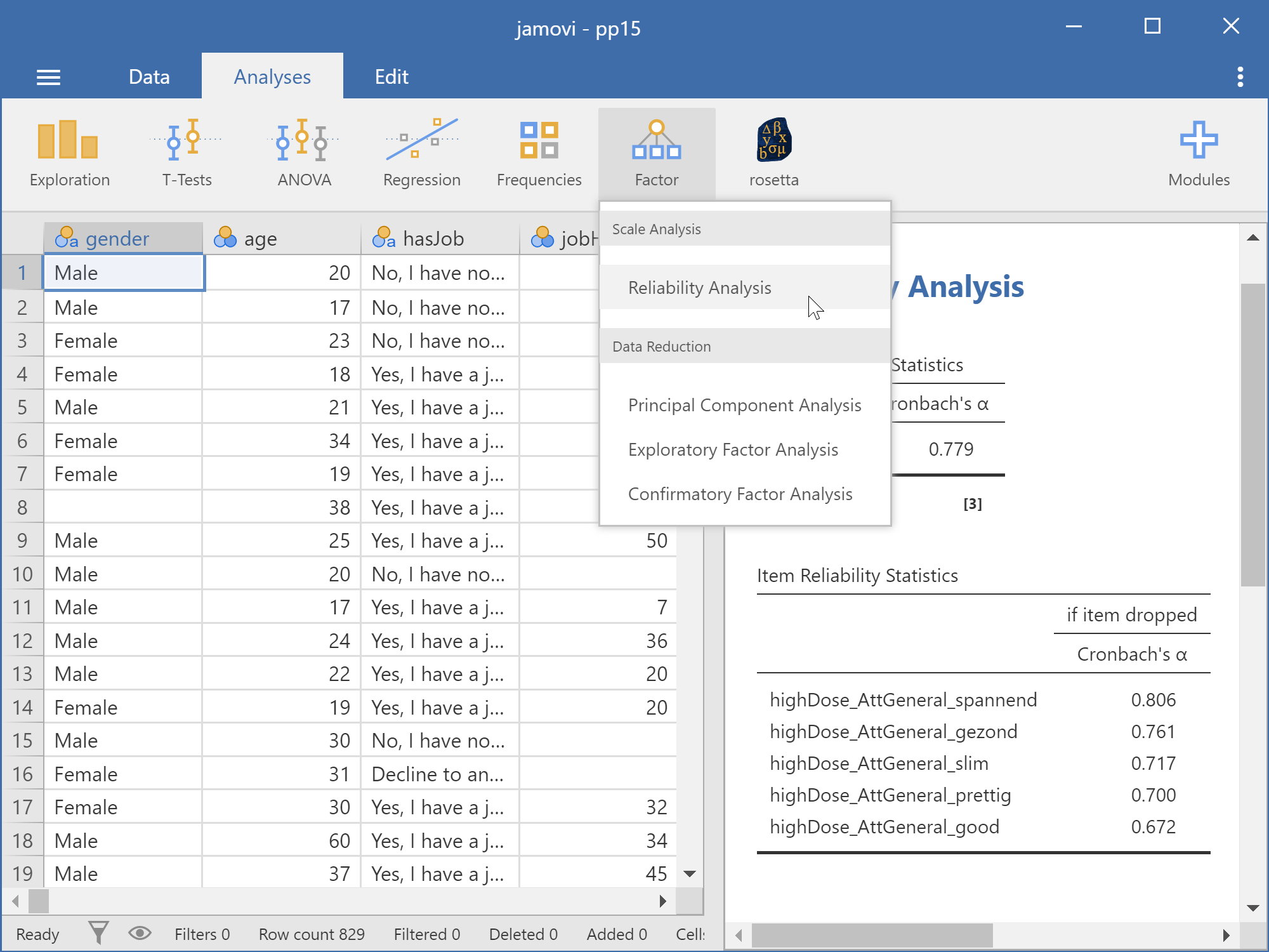
Figure 17.1: Opening the reliability analysis menu in jamovi
In the box at the left, select all variables you want to include in this analysis and move them to the box labelled “Items” using the button labelled with the rightward-pointing arrow as shown in Figure 17.2.
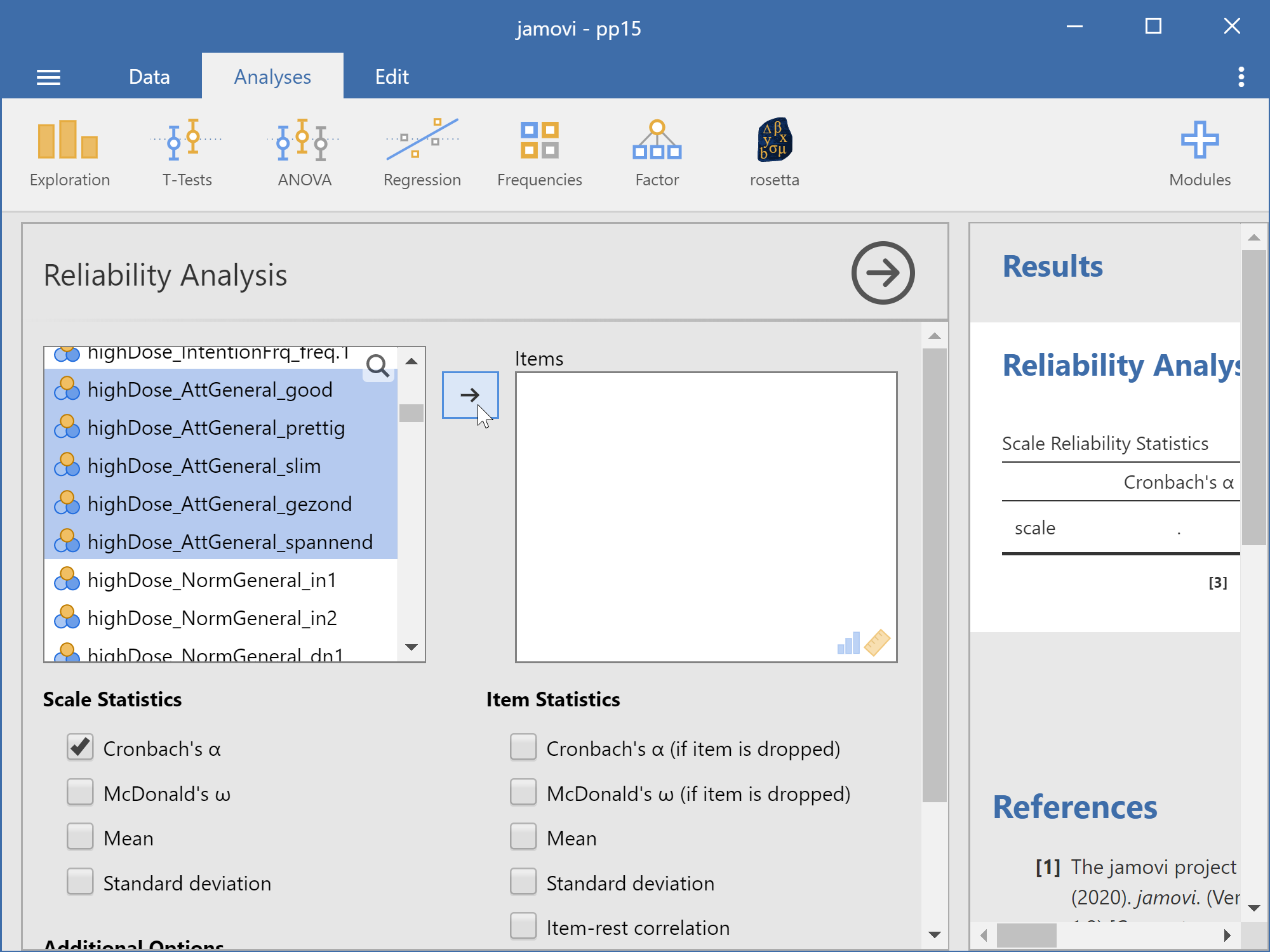
Figure 17.2: Adding the items to analyse in jamovi
You can now select which options you want by checking more checkboxes and indicating other settings in the left-hand panel. You will immediately see the results in the right-hand panel update as shown in Figure 17.3.
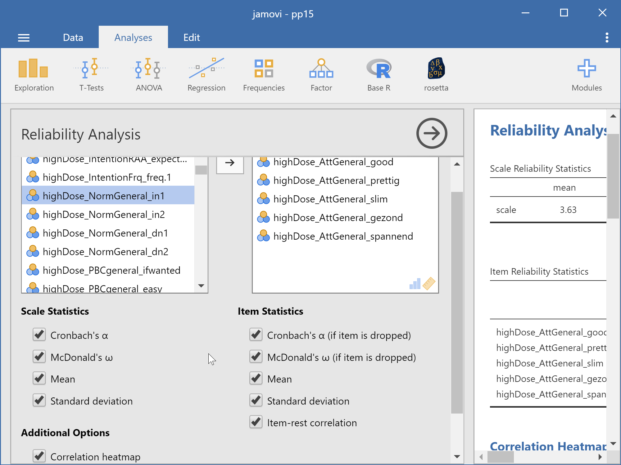
Figure 17.3: Adding the items to analyse in jamovi
17.3 Input: R
17.3.1 R: rosetta
In R, using the rosetta package, you can use the following command:
rosetta::reliability(
  data = dat,
  items = c(
    "highDose_AttGeneral_good"
    "highDose_AttGeneral_prettig"
    "highDose_AttGeneral_slim"
    "highDose_AttGeneral_gezond"
    "highDose_AttGeneral_spannend"
  )
);
To order additional information, such as descriptive statistics, inter-item correlations, and other scale statistics, you can specify additional options. You can also specify item labels to print instead of the variable names:
rosetta::reliability(
data = dat,
items = c(
"highDose_AttGeneral_good",
"highDose_AttGeneral_prettig",
"highDose_AttGeneral_slim",
"highDose_AttGeneral_gezond",
"highDose_AttGeneral_spannend"
),
itemLabels = c(
"Attitude: good",
"Attitude: pleasant",
"Attitude: smart",
"Attitude: healthy",
"Attitude: exciting"
),
descriptives = TRUE,
itemLevel = TRUE,
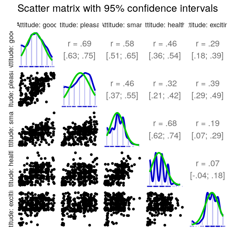
scatterMatrix = TRUE,
itemOmittedCorsWithRest = TRUE,
alphaOmittedCIs = TRUE
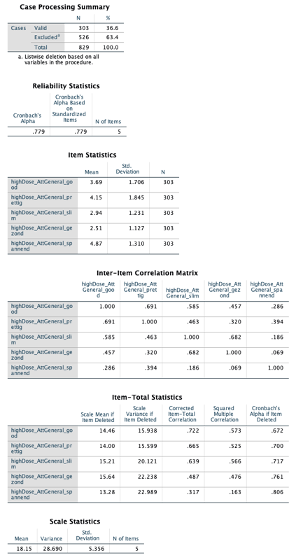
);17.4 Input: SPSS
In SPSS, you can use the following command:
RELIABILITY
  /VARIABLES =
    highDose_AttGeneral_good
    highDose_AttGeneral_prettig
    highDose_AttGeneral_slim
    highDose_AttGeneral_gezond
    highDose_AttGeneral_spannend
  /MODEL = ALPHA.
To order additional information, such as descriptive statistics, inter-item correlations, and other scale statistics, you can specify additional options:
RELIABILITY
  /VARIABLES =
    highDose_AttGeneral_good
    highDose_AttGeneral_prettig
    highDose_AttGeneral_slim
    highDose_AttGeneral_gezond
    highDose_AttGeneral_spannend
  /MODEL = ALPHA
  /STATISTICS = DESCRIPTIVE SCALE CORR
  /SUMMARY = TOTAL.
17.6 Output: R
17.6.1 Reliability analysis
17.6.1.1 Scale structure
17.6.1.1.1 Scale structure
17.6.1.1.1.1 Information about this scale
| Dataframe: | res$data |
| Items: | highDose_AttGeneral_good, highDose_AttGeneral_prettig, highDose_AttGeneral_slim, highDose_AttGeneral_gezond & highDose_AttGeneral_spannend |
| Observations: | 303 |
| Positive correlations: | 10 |
| Number of correlations: | 10 |
| Percentage positive correlations: | 100 |
17.6.1.1.1.2 Estimates assuming interval level
| Omega (total): | 0.79 |
| Omega (hierarchical): | 0.80 |
| Revelle’s Omega (total): | 0.79 |
| Greatest Lower Bound (GLB): | 0.87 |
| Coefficient H: | 0.85 |
| Coefficient Alpha: | 0.78 |
Note: the normal point estimate and confidence interval for omega are based on the procedure suggested by Dunn, Baguley & Brunsden (2013) using the MBESS function ci.reliability, whereas the psych package point estimate was suggested in Revelle & Zinbarg (2008). See the help (‘?ufs::scaleStructure’) for more information.
17.6.1.2 Scale descriptives
| Mean, 95% CI lower bound: |
Mean, point estimate: |
Mean, 95% CI upper bound: | SD, 95% CI lower bound: |
SD, point estimate: |
SD, 95% CI upper bound: | |
|---|---|---|---|---|---|---|
| scale | 3.51 | 3.63 | 3.75 | 0.99 | 1.07 | 1.16 |
17.6.1.3 Item-level descriptives
| Mean, 95% CI lower bound: |
Mean, point estimate: |
Mean, 95% CI upper bound: | SD, 95% CI lower bound: |
SD, point estimate: |
SD, 95% CI upper bound: | |
|---|---|---|---|---|---|---|
| Attitude: good | 3.49 | 3.69 | 3.88 | 1.58 | 1.71 | 1.85 |
| Attitude: pleasant | 3.94 | 4.15 | 4.35 | 1.71 | 1.84 | 2.00 |
| Attitude: smart | 2.80 | 2.94 | 3.08 | 1.14 | 1.23 | 1.34 |
| Attitude: healthy | 2.38 | 2.51 | 2.64 | 1.04 | 1.13 | 1.22 |
| Attitude: exciting | 4.72 | 4.87 | 5.02 | 1.21 | 1.31 | 1.42 |
17.6.1.4 Correlations of items with scale
|
Item-rest correlations: 95% CI lower bound |
Item-rest correlations: point estimate |
Item-rest correlations: 95% CI upper bound |
|
|---|---|---|---|
| Attitude: good | 0.66 | 0.72 | 0.77 |
| Attitude: pleasant | 0.60 | 0.66 | 0.72 |
| Attitude: smart | 0.57 | 0.64 | 0.70 |
| Attitude: healthy | 0.40 | 0.49 | 0.57 |
| Attitude: exciting | 0.21 | 0.32 | 0.42 |
17.6.1.5 Internal consistency estimates with items omitted
|
Coefficient Alpha: 95% CI lower bound |
Coefficient Alpha: point estimate |
Coefficient Alpha: 95% CI upper bound |
Omega (from psych):point estimate |
|
|---|---|---|---|---|
| Attitude: good | 0.61 | 0.67 | 0.73 | 0.72 |
| Attitude: pleasant | 0.64 | 0.70 | 0.75 | 0.75 |
| Attitude: smart | 0.66 | 0.72 | 0.76 | 0.73 |
| Attitude: healthy | 0.72 | 0.76 | 0.80 | 0.78 |
| Attitude: exciting | 0.77 | 0.81 | 0.84 | 0.82 |