Chapter 24 Simple Regression Analysis

24.1 Intro

Univariate regression analysis (with one predictor) can be useful to get an estimate of the increase in the dependent variable as a function of the predictor variable. The approach differs for continuous or categorical predictors, and both will be shown.

24.1.1 Example dataset

This example uses the Rosetta Stats example dataset “pp15” (see Chapter 1 for information about the datasets and Chapter 3 for an explanation of how to load datasets).

24.1.2 Variable(s)

From this dataset, this example uses variables xtcUseDosePref as dependent variable (the MDMA dose a participant prefers), highDose_attitude as a continuous predictor (the attitude towards using a high dose of MDMA), and hasJob as a categorical predictor.

24.2 Input: jamovi

In the “Analyses” tab, click the “Regression” button and from the menu that appears, select “Linear Regression” as shown in Figure 24.1.

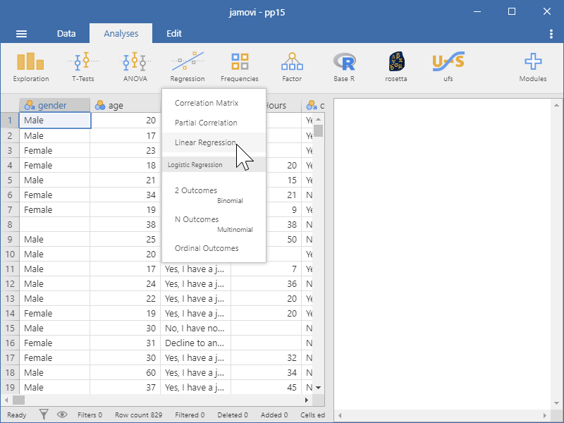
Figure 24.1: Opening the linear regression menu in jamovi

In the box at the left, select the dependent variable and move it to the box labelled “Dependent variable” using the button labelled with the rightward-pointing arrow as shown in Figure 24.2.

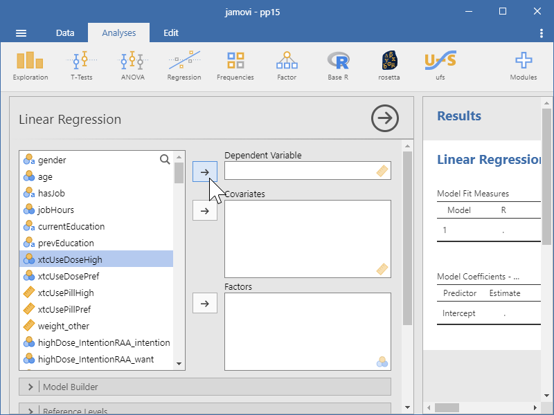
Figure 24.2: Selecting the dependent variable for the regression analysis in jamovi

Then, select the predictor variable and move it to the box labelled “Covariates” if it is a continuous variable, and to the box labelled “Factors” if it is a categorical variable, as shown in Figure 24.3.

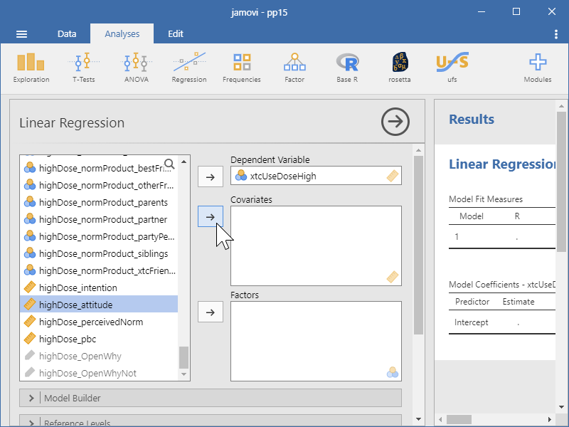
Figure 24.3: Selecting the predictor for the regression analysis in jamovi

The results will immediately be shown in the right-hand “Results” panel. You can scroll down to specify additional analyses, for example to order more details about the coefficient by opening the “Model Coefficients” section as shown in Figure 24.4.

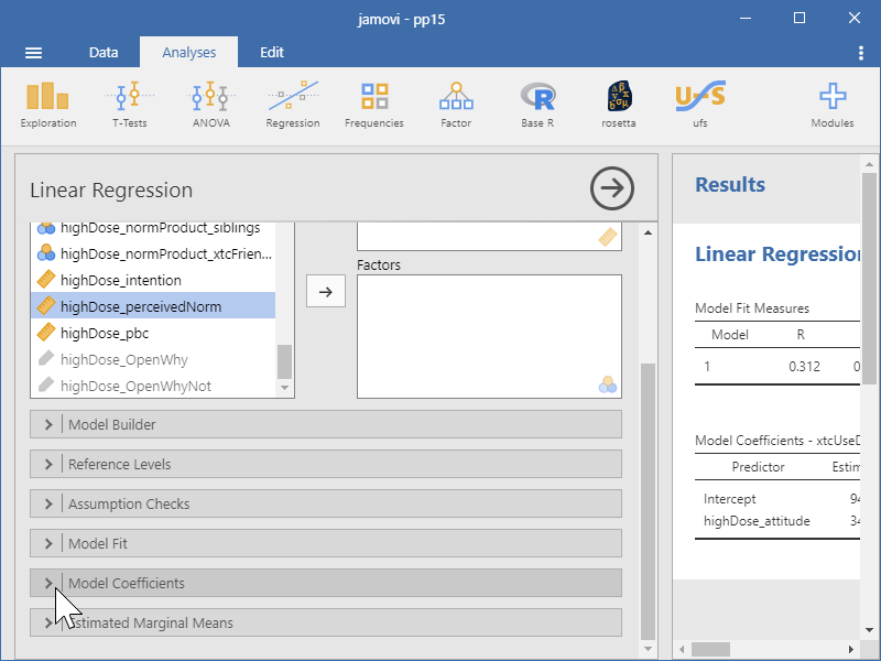
Figure 24.4: Opening the Model Coefficients section in jamovi

For example, to request the confidence interval for the slope coefficient and the standardized (scaled) coefficient, check the corresponding check boxes as shown in Figure 24.5.

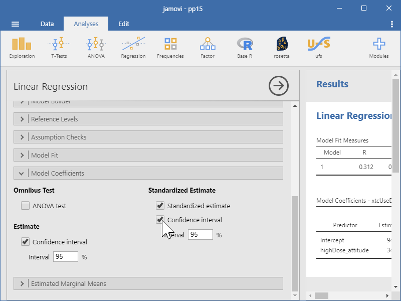
Figure 24.5: Selecting the predictor for the regression analysis in jamovi

24.3 Input: R

In R, there are roughly three approaches. Many analyses can be done with base R without installing additional packages. The rosetta package accompanies this book and aims to provide output similar to jamovi and SPSS with simple commands. Finally, the tidyverse is a popular collection of packages that try to work together consistently but implement a different underlying logic that base R (and so, the rosetta package).

24.3.1 R: base R

In base R, the lm (linear model) function can be combined with the summary function to show the most important results. With a continuous predictor, the code is as follows.

result <-
  lm(
    xtcUseDosePref ~ highDose_attitude,
    data=dat
  );
summary(
  result
);

With a categorical predictor, the code is essentially the same, since R automatically treats variables that are factors as categorical, and numeric vectors as continuous variables.

result <-
  lm(
    xtcUseDosePref ~ hasJob,
    data=dat
  );
summary(
  result
);

24.3.2 R: rosetta

In the rosetta package, the regr function wraps base R’s lm function to present output similar to that provided by other statistics programs in one command.

rosetta::regr(
  xtcUseDosePref ~ highDose_attitude,
  data=dat
);

Like lm in base R, the command is the same for a continuous predictor as it is for a categorical predictor (i.e. by replacing highDose_attitude with hasJob).

A scatter plot can be requested using argument plot=TRUE):

rosetta::regr(
  xtcUseDosePref ~ highDose_attitude,
  data=dat,
  plot=TRUE
);

24.4 Input: SPSS

For SPSS, there are two approaches: using the Graphical User Interface (GUI) or specify an analysis script, which in SPSS are called “syntax”.

24.4.1 SPSS: GUI

Figure 24.6: A screenshot placeholder

24.4.2 SPSS: Syntax

In SPSS, the REGRESSION command is used (don’t forget the period at the end (.), the command terminator):

REGRESSION
  /DEPENDENT
    xtcUseDosePref
  /METHOD
    ENTER highDose_attitude 
  /STATISTICS
    COEF
    CI(95)
    R
    ANOVA
.

With a categorical predictor the code is essentially the same, since SPSS “sees” whether the predictor is continuous or categorical.

REGRESSION
  /DEPENDENT
    xtcUseDosePref
  /METHOD
    ENTER gender
  /STATISTICS
    COEF
    CI(95)
    R
    ANOVA
.

24.5 Output: jamovi

Figure 24.7: Univariate regression analysis output in jamovi

24.6 Output: R

24.6.1 R: base R


Call:
lm(formula = xtcUseDosePref ~ highDose_attitude, data = pp15)

Residuals:
    Min      1Q  Median      3Q     Max 
-144.58  -58.56  -11.85   41.44  348.60 

Coefficients:
                  Estimate Std. Error t value Pr(>|t|)    
(Intercept)         56.394     24.890   2.266   0.0251 *  
highDose_attitude   32.956      6.704   4.916 2.56e-06 ***
---
Signif. codes:  0 '***' 0.001 '**' 0.01 '*' 0.05 '.' 0.1 ' ' 1

Residual standard error: 88.8 on 133 degrees of freedom
  (694 observations deleted due to missingness)
Multiple R-squared:  0.1538,    Adjusted R-squared:  0.1474 
F-statistic: 24.16 on 1 and 133 DF,  p-value: 2.559e-06

24.6.2 R: rosetta

24.6.2.1 Regression analysis

Summary

Formula:	xtcUseDosePref ~ highDose_attitude
Sample size:	135
Multiple R-squared:	[.06; .28] (point estimate = 0.15, adjusted = 0.15)
Test for significance: (of full model)	F[1, 133] = 24.16, p < .001

Raw regression coefficients

	95% conf. int.	estimate	se	t	p
(Intercept)	[7.16; 105.63]	56.39	24.89	2.27	.025
highDose_attitude	[19.7; 46.22]	32.96	6.70	4.92	<.001
^a These are unstandardized beta values, called ‘B’ in SPSS.

Scaled regression coefficients

	95% conf. int.	estimate	se	t	p
(Intercept)	[-0.05; 0.25]	0.10	0.08	1.32	.188
highDose_attitude	[0.21; 0.5]	0.36	0.07	4.92	<.001
^a These are standardized beta values, called ‘Beta’ in SPSS.

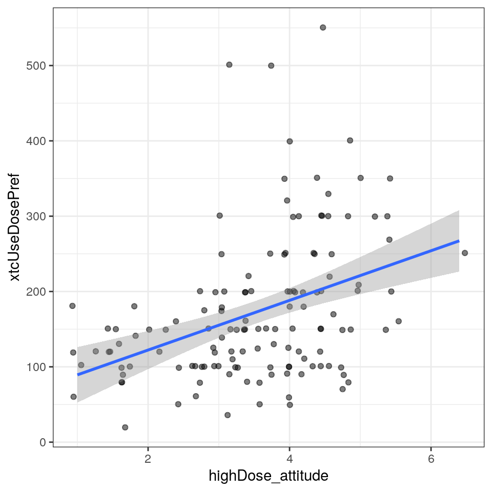
Figure 24.8: Scatterplot with regression line